Detecting missing data with z-scores

Introduction

When loading time-series data into a data warehouse, you typically want to verify that you have successfully loaded all the data that you would expect. You typically put checks all along your ingestion pipeline, but you can never be sure that everything succeeded until you check the last model. So how do you check for missing data?

If you know exactly the number of rows that you expect each day, problem solved, nothing to see here. However if you don't, statistical methods can help detect anomalies in the time series and identify missing data. This article will focus on detecting missing rows based solely on the number of rows by day, making this approach flexible to any kind of time series.

Consider a Snowflake table containing portfolio valuation data, at holding level, for each business day. The method should be robust to adding holdings or portfolios in the table, thus we are expecting the number of rows to increase occasionally, especially as I am making the assumption that duplicates can be flagged by other tests. We'll first discuss of mathematical constructs to achieve this, and then we'll think of some SQL code.

Fundamental principles

To detect missing data in a time series, we use a core principle of Time-Series Anomaly Detection to check whether data points deviate significantly from an established pattern or trend. Two crucial concepts to achieve this are Z-score and Moving Average.

The moving average is the average of the data points in a time window sliding along the time axis. It is used to smooth out short-term fluctuations and highlight long-term trends and cycles. For example, if the time window is 7 days, the moving average at a certain time point would be the average of that day and the six preceding days. In SQL, this is achieved with windows functions.

The z-score is a statistical measurement that describes a value's relationship to the mean of a group of values. The Z-score is measured in terms of standard deviations from the mean. If a Z-score is 0, it indicates that the data point's score is identical to the mean score. A Z-score of 1.0 would indicate a value that is one standard deviation from the mean. The z-score is signed, so that we can know if the data point is below or above the average.

We will apply both of these techniques in the following way:

1. Calculate "daily_rows": the daily number of rows in the table.
2. Calculate the moving average of "daily_rows" over a suitable time window (say, the past 7 days).
3. Compute the standard deviation of "daily_rows" in the same window.
4. Calculate the Z-score for each day's "daily_rows". This will be (daily_rows - moving average) / standard deviation.
5. If the Z-score is less than a certain threshold (say, -2), flag it as a potential anomaly. This means the "daily_rows" is significantly lower than what we'd expect based on recent trends, suggesting that data may be missing.

First try

with portfolio_table as (
    select * from 'nav.csv'
),
daily_counts as (
    select 
        market_date as date, 
        count(*) as daily_rows
    from portfolio_table 
    group by market_date
),
moving_averages as (
    select 
        date,
        daily_rows,
        avg(daily_rows) over (
            order by date asc rows between 7 preceding and current row
        ) as moving_avg,
        stddev(daily_rows) over (
            order by date asc rows between 7 preceding and current row
        ) as moving_stddev,
        -- we'll add this for debugging/understanding
        lag(daily_rows) over (
            order by date asc
        ) as previous_count
    from daily_counts
),
z_scores as (
    select 
        date,
        (daily_rows - moving_avg) / nullif(moving_stddev, 0) as z_score,
        abs(daily_rows - moving_avg) / nullif(moving_avg, 0) as relative_deviation,
        * -- those are only needed for debugging
    from 
        moving_averages
)
select 
    date,
    z_score
from z_scores
where 
    z_score < -2
order by date

To see whether this is doing a good job, we'll generate some fake data to model. We could simply generate a fake sequence of daily_counts, but to see it in full action end-to-end, let's actually model some market data. For this, we'll use R.

Generating the data with R

install.packages(c("tidyverse", "lubridate"))
# set seed for reproducibility
set.seed(42)
# generate portfolio data
portfolios <- paste("Portfolio", LETTERS[1:5])

# generate holding data
holdings <- paste("Holding", seq(1:50))
# generate 3 months of dates
dates <- seq(as.Date("2023-01-01"), as.Date("2023-03-31"), by = "day")

# generate a slow increase in number of rows for each day
num_rows <- round(runif(length(dates), min = 50, max = 55)) + seq_along(dates) * 0.02
num_rows <- round(num_rows)

# pick a random day in the second month for the jump
jump_date <- sample(32:59, 1)

# double the number of rows from the jump date
num_rows[jump_date:length(num_rows)] <- num_rows[jump_date:length(num_rows)] * 2

df <- tibble(
  market_date = rep(dates, times = num_rows),
  portfolio = sample(portfolios, sum(num_rows), replace = TRUE),
  holding = sample(holdings, sum(num_rows), replace = TRUE),
  weight = runif(sum(num_rows), min = 0.01, max = 0.1),
  shares = pmax(rnorm(sum(num_rows), mean = 5000, sd = 1000), 0),
  price = rnorm(sum(num_rows), mean = 100, sd = 20)
)

write.csv(df, file = "nav.csv")

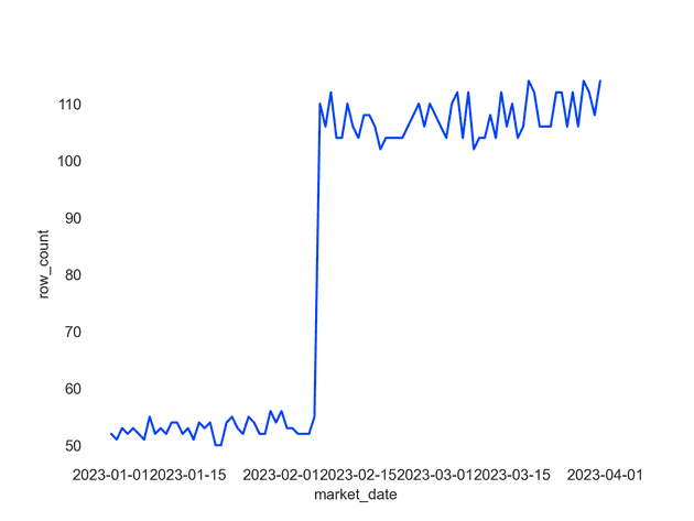
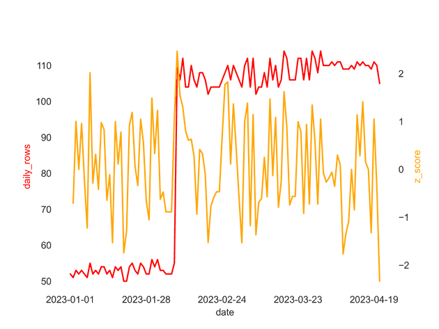
This gets us the following daily counts:

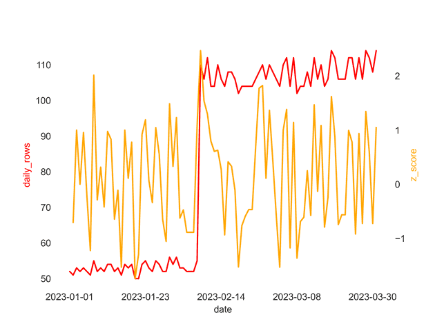
Analysis

Because we only care about decreases, we can see that row jumps are not marked as anomalies, because they have a large positive z-score, which is what we want in our case.

Missing data example

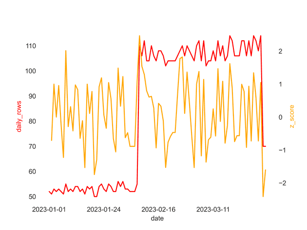
So far so good, but there is not anomaly to detect yet. Let's add a single day with missing data by directly ingesting into the daily_counts:

daily_counts as (
    select 
        market_date as date, 
        count(*) as daily_rows
    from portfolio_table 
    group by market_date
    union all
    select '2023-04-01' as market_date, 20 as daily_rows
),

We can see now that this row is rightfully flagged as an anomaly, and we are able to detect missing data for that date. Now this is a nice example, it may not always be easy to choose the right z-score threshold and window size. At the end of the day, this is a trade-off between false positives and false negatives.

The choice of the Z-score threshold is determined by how sensitive you want your anomaly detection to be. A Z-score threshold of -2 indicates that any daily row count more than 2 standard deviations below the moving average will be flagged as an anomaly. The more negative the Z-score threshold, the less sensitive the anomaly detection (fewer anomalies will be flagged).

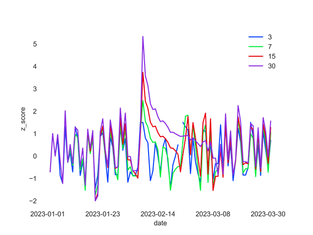
The window size represents the length of the time period you consider as "normal" for your data. It is used to calculate the moving average and standard deviation. If your data has strong weekly seasonality (e.g. weekdays always have more rows than weekends), you might use a 7-day window size. If your data has strong monthly patterns, you might use a 30-day window size. Smaller window sizes will make the anomaly detection more sensitive to recent changes, while larger window sizes will make it less sensitive to recent changes.

On the false positive side, there is one more pathological case to be taken into account that should force us to improve our anomaly condition. If we use only the z-score we see that we can get pathological cases where the standard deviation is so small that the tiniest variation causes the z-score to explode. When the data has very low variance, like being exactly the same for a week, even a small deviation from the norm can result in a high absolute Z-score. One approach to manage this issue would be to use a modified Z-score which is based on the median absolute deviation (MAD) instead of the standard deviation. The modified Z-score is more robust against outliers.

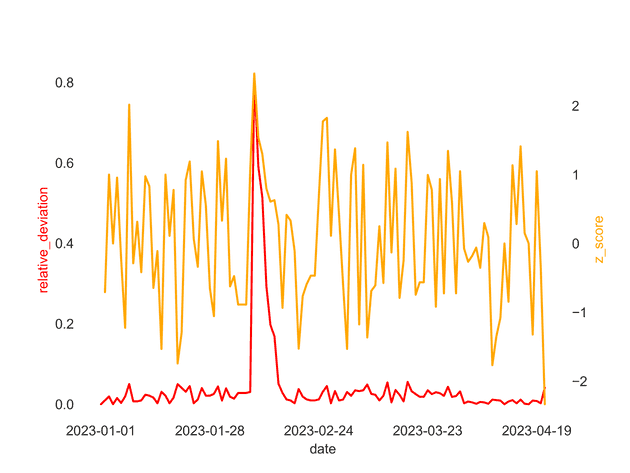
Alternatively, we can add a relative measure of deviation, for example by also considering the percentage deviation from the moving average. If the percentage deviation is small, we might choose not to flag it as an anomaly even if the Z-score is below our threshold. This would help to prevent small absolute changes from being flagged as anomalies when the standard deviation is very low.