Tyres Surface temperature estimation in iRacing

Understanding tyres is crucial in motorsport. A few months ago we have Kimi, leader of the F1 championship, ask in a panicked voice to his race engineer Bono, if his tyres are cooked as he’s losing performance (grip), to which he replies, no it’s just surface temps. The implication is that by cooling the tyres, Kimi can recover the performance, just showing how crucial understanding tyres are.

There are obviously many things happening inside a tyre at once, but that small exchange captures an important distinction. A driver can suddenly lose grip because the surface has become too hot without the tyre necessarily being permanently gone. Get it back into a healthier temperature range and some of that performance can come back. For a race engineer, understanding why grip disappeared matters almost as much as knowing that it disappeared in the first place.

iRacing is the reference in terms of sim racing (ultra realistic motorsport games), and while it provides a ton of data that can be exported (understanding telemetry traces is a great tool to get faster), live surface temps are not available. I am building an AI race engineer (my Bono), and this information is then lacking during races. I arbitrarely setup a target of 2°C, thinking that I’d definitely be OK with that error, for racing diagnostics that difference has no impact.

There’s then an incentive to estimate tyre temps, both to add a diagnostic tool to the race engineer, and as a fun intellectual exercise. More concretely, the question becomes: can we reconstruct tyre surface temperatures accurately enough from the telemetry that is available live?

This is important because I’m not trying to build a perfect tyre simulator. If the real temperature is 103°C and my race engineer thinks it’s 104°C, I don’t care. The useful output is something closer to: the front-right is overheating because you’ve been abusing it for the last few corners, or the spike from the lockup is now cooling down and the tyre should recover. That gives the problem a much more practical definition of success.

Collecting the first data

First step is collecting baseline training data and analyzing what’s even available.

The nice thing with iRacing is that there is no shortage of telemetry. Steering angle, throttle, brake pressure, accelerations, velocities, tyre information and a huge number of other channels can all be recorded. For training, I can also use information that isn’t available to the live race engineer: the true tyre surface temperatures become my labels.

The slightly dangerous part is that this makes it easy to accidentally solve a different problem from the one I actually care about.

Everything was done with agentic coding, so I had to enforce that we only used live channels. Wheel speeds are a very attractive training signal: compared with car velocity, they’re a close proxy for slip, which tells us how much the tyres are “rubbing on the floor” and heating up. Unfortunately, they’re only available after the session in a disk dump.

This is exactly the sort of mistake that agentic coding makes easier. You ask the agent to find the channels most correlated with tyre temperature, it finds a fantastic signal, and you train a model that works suspiciously well — only to discover that the signal doesn’t exist where the model is meant to run.

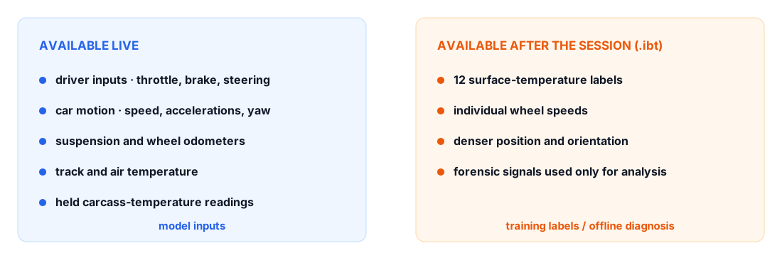
Finding out that wheel speeds weren’t available live was a bit of a heart-sinking moment. They were the most direct way to estimate slip, and without them it wasn’t obvious that the problem would still be learnable. My hope was that the model could recover those relationships indirectly from the driving inputs and car dynamics, with odometers — how much distance each individual wheel has travelled — providing one alternative signal.

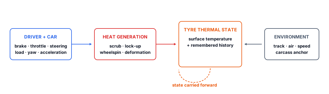
Slip is attractive because it gives us an intuitive bridge between driving and temperature. A tyre rolling cleanly along the road is one situation; a tyre being dragged sideways through a corner, spinning under power, or locking under braking is another. In all of those cases, mechanical energy is dissipated at the contact patch.

Even without a perfect slip signal, many of its causes are observable. We know what the driver is asking through steering, throttle and brake, how the car is accelerating and rotating, and what each wheel has travelled over time. The question is whether those weaker signals contain enough information for the model to reconstruct what the missing wheel-speed channel would have made much easier.

Beyond estimating how much energy we’re putting into the tyre through slip, the other big thing the model has to learn is what I think of as tyre inertia: tyre temperature has memory. Heat builds up and dissipates progressively, so the current surface temperature depends not only on what the car is doing now, but on what the tyre has been through over the preceding seconds.

That mental picture ended up being useful throughout the project. You can abuse a tyre for a few seconds, stop doing it, and the temperature doesn’t magically snap back to where it started. Likewise, one instant of braking doesn’t tell you very much without knowing whether the tyre entered the braking zone already hot or cold.

There are therefore roughly two parts to the problem:

• heat generation: what is happening at the tyre right now that puts energy into it;
• thermal inertia: given its previous state, how quickly does that heat accumulate or disappear?

The second part is why treating every telemetry sample independently was never going to be enough.

A deliberately simple baseline

Before moving on to a recurrent model, I built a deliberately simple baseline with classical linear regression. The idea was to represent tyre temperature as heat coming in minus heat going out, with the previous temperature providing a basic form of thermal inertia.

For each tyre zone, the fitted temperature rate was:

$$\begin{aligned} \dot{T}_s ={}& \sum_j \beta_j H_j \\ &+ \beta_c(T_c - T_s) \\ &+ \beta_r(T_{\mathrm{track}} - T_s) \\ &+ \beta_a(T_{\mathrm{air}} - T_s) \\ &+ \beta_v\,v(T_{\mathrm{air}} - T_s), \qquad \beta_\bullet \geq 0 \end{aligned}$$

where $H_j$ contains the rolling slip, brake, suspension, cornering and steering heat proxies. The remaining terms model heat exchange with the carcass, track and air, including speed-dependent cooling. One non-negative least-squares model was fitted per tyre zone, then rolled forward one sample at a time:

$$\begin{aligned} T_{s,t+\Delta t} ={}& \operatorname{clip}\!\bigl( \\ &T_{s,t} + \Delta t\, \operatorname{clip}(\dot{T}_{s,t}, -60, 80), \\ &-40, 350 \bigr) \end{aligned}$$

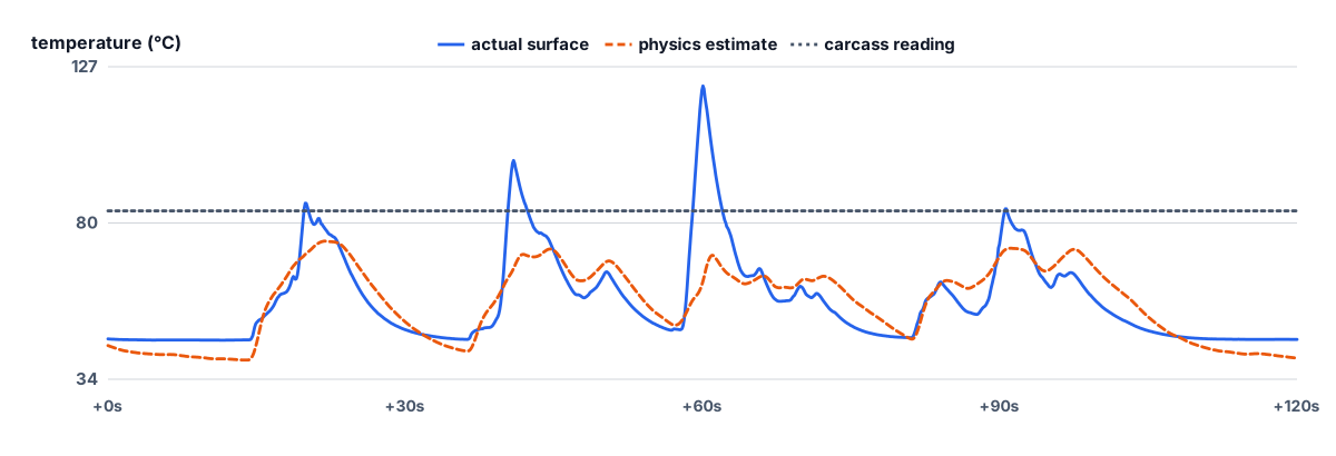
It was never expected to be especially accurate, but it gave me a useful reference point and confirmed that the live telemetry contained enough information to estimate temperature at all. The model could follow the broad direction of the temperature traces — heating under sustained load and cooling afterwards — but it struggled with the size and timing of individual events.

That made the next step fairly obvious: the model needed to learn a richer internal state, rather than relying on a hand-designed approximation of the tyre’s thermal behaviour.

Moving to a GRU

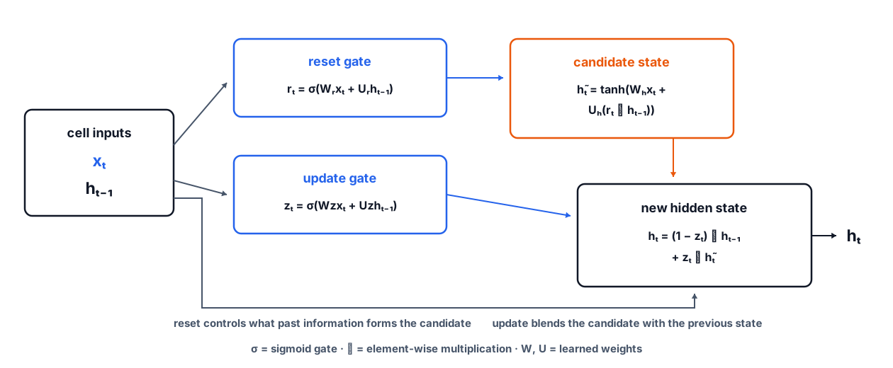
The obvious next choice is a GRU RNN. Tyre temperature is inherently stateful, and GRUs are specifically built to learn from sequences while retaining useful information over long horizons: their gates let the model decide how much of its existing hidden state to preserve and how much to update from new inputs. That makes them particularly attractive for learning the “tyre inertia” part of the problem, while remaining simpler than an LSTM.

In other words, instead of me explicitly deciding how quickly a tyre should forget what happened five or ten seconds ago, the recurrent state gives the network a mechanism to learn that behaviour.

That maps surprisingly neatly onto the mental picture of tyre inertia.

Setting	Selected GRU
Sampling	10 Hz, with causal aggregation inside each 100 ms bin
Training window	30 seconds / 300 samples
Window stride	5 seconds
Input	49 normalised live telemetry features, plus the sample interval
Recurrent core	One GRU layer with 128 hidden units
Output	12 continuous temperatures at every sample: left, middle and right for all four tyres
Prediction form	Direct temperature in °C, not a rate or delta
Parameters	70,668

The first training is very promising, but there is still substantial residual error — especially around cooling events — and we immediately notice what would become the key challenge of the project, which was pretty obvious in retrospect: class, or rather regime imbalance.

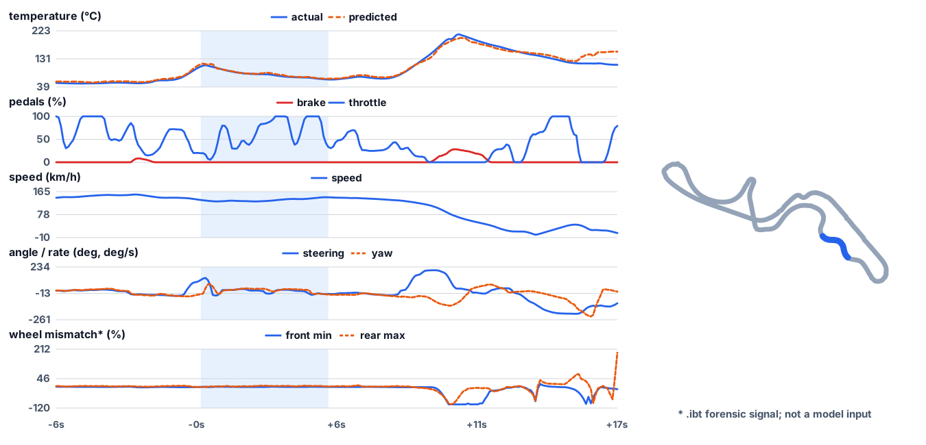
The average performance is encouraging enough that simply looking at an aggregate metric can actually be misleading. During ordinary laps, large portions of the prediction can sit remarkably close to reality. Then one unusual event happens and the model suddenly misses a large temperature excursion.

That distinction matters a lot for the final application. A race engineer that predicts boring laps perfectly but becomes unreliable exactly when I lock a tyre or start sliding is not doing the part of the job I care about most.

The hard parts are rare

Most drivers of a reasonable level, including me, spend most of a lap driving relatively normally. That doesn’t mean flawless driving, but it means we’re rarely putting a tyre under sustained, extreme stress. The events that do — lockups, slides, some high-speed corners, and their front/rear variants — are comparatively rare, while producing some of the most difficult extreme temperature spikes for the model to learn.

Unfortunately, those rare regimes are also exactly where the model makes some of its largest errors.

The dataset is therefore imbalanced in a slightly awkward way. This isn’t classification where 95% of the examples belong to class A and 5% to class B. Every sample is still just another point in a continuous time series. But qualitatively, the driving falls into very different regimes.

Thousands of samples might represent tyres behaving normally through an ordinary lap. Then a lockup produces a very distinctive sequence over only a few seconds. The optimizer has a lot more opportunities to get rewarded for shaving a tiny amount of error off normal driving than for correctly learning an event that barely appears in the dataset.

And the rare events aren’t merely uncommon versions of the normal ones. They often create the sharpest shapes in the entire temperature trace.

←

→

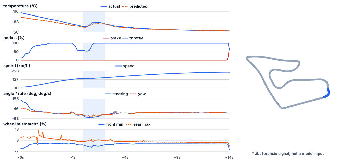
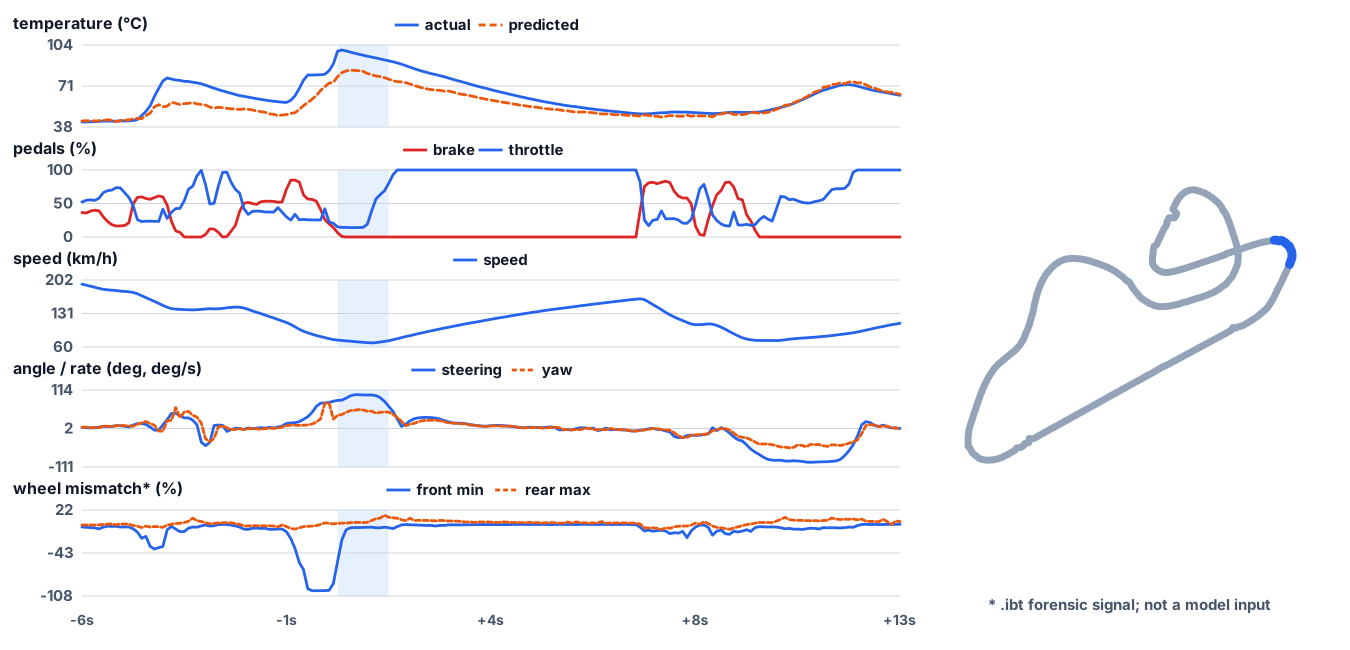
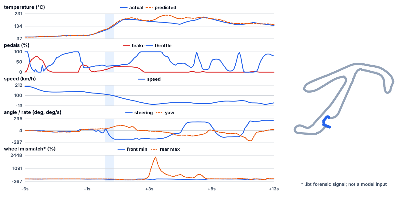
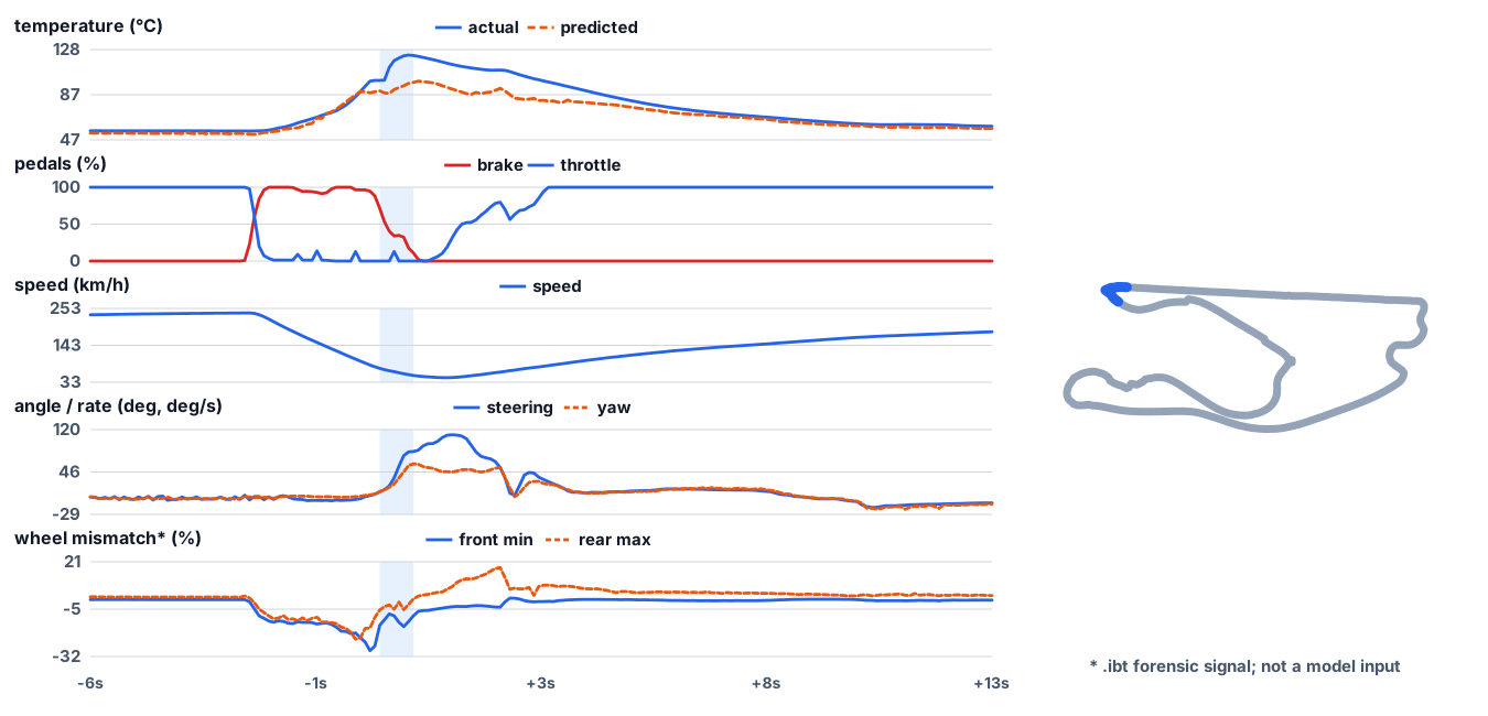
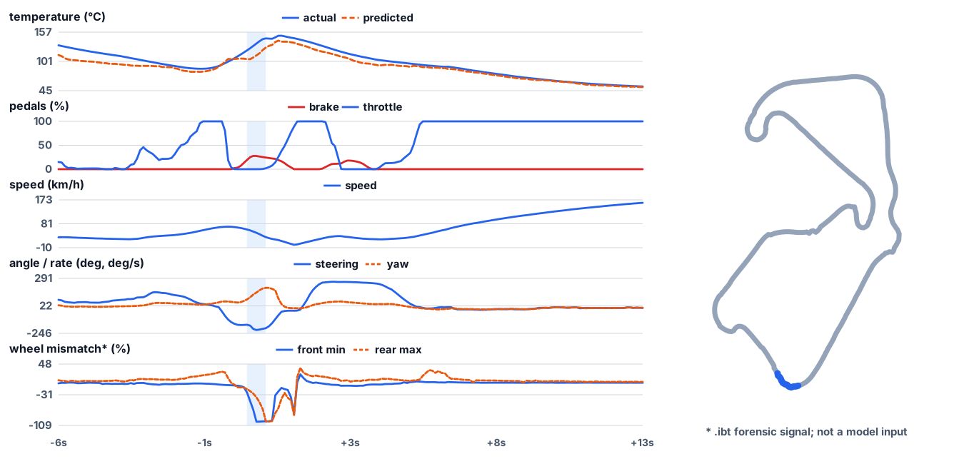
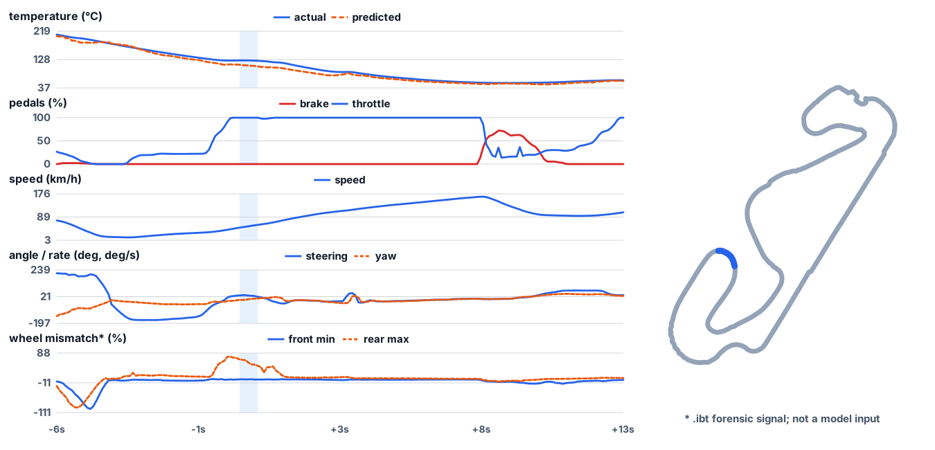
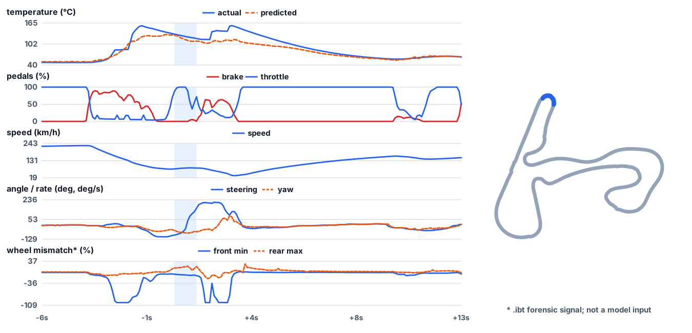
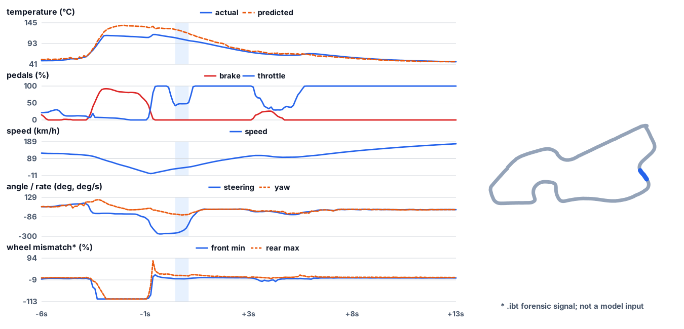
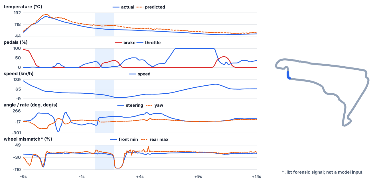
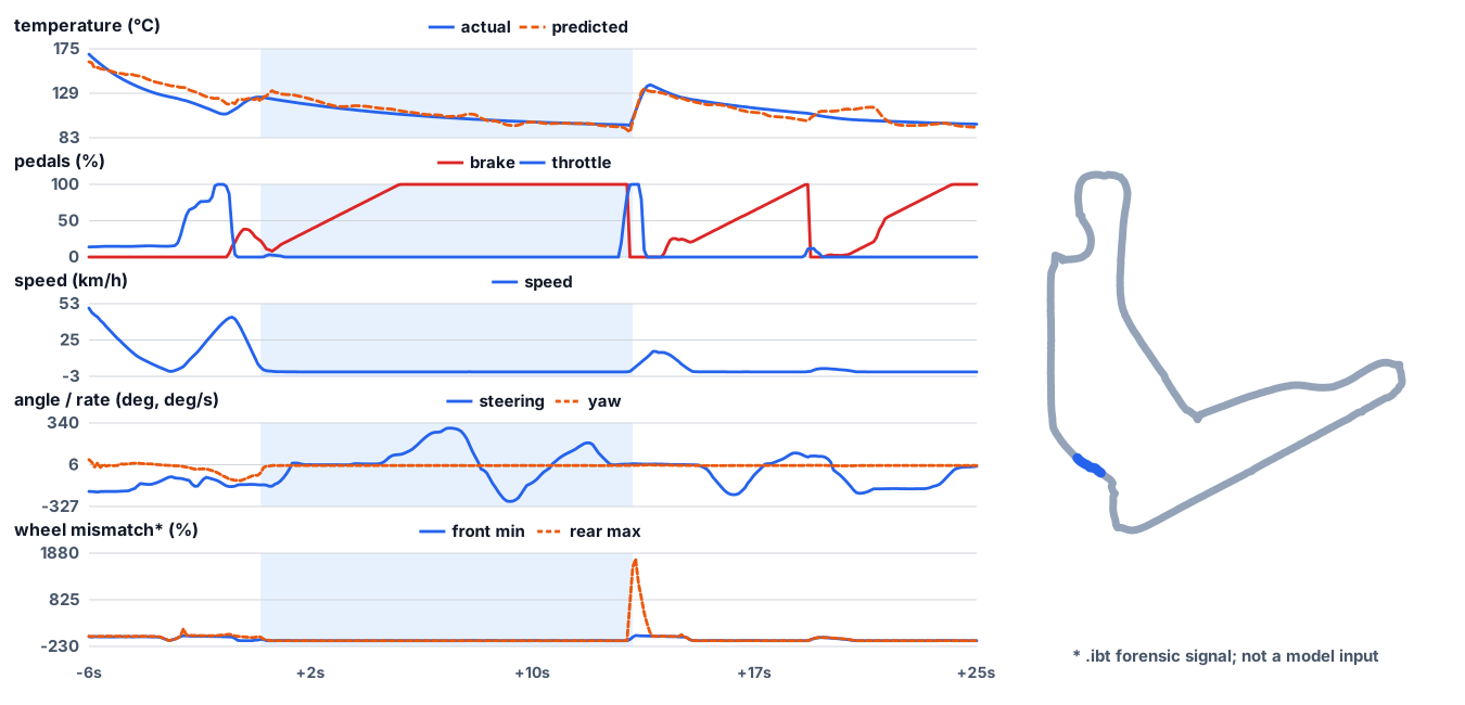
This also makes the usual train/test metric harder to interpret. A randomly selected test set will mostly contain ordinary driving because the original dataset mostly contains ordinary driving. A model can therefore improve its headline metric while remaining mediocre on exactly the events I want the race engineer to diagnose.

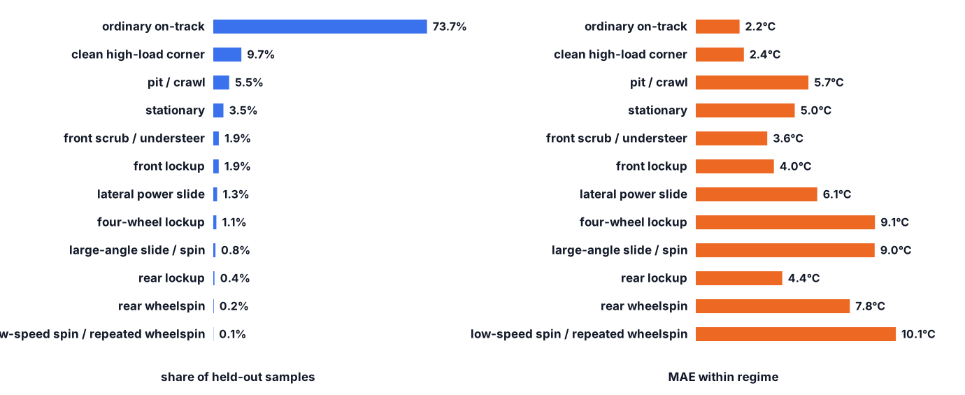
Car setup, brake shapes and driving style introduce another source of variation — there are fundamentally different ways of driving a racing car, from relatively understeery to oversteery approaches — although this doesn’t appear to be what’s causing the largest errors.

A front-biased setup may naturally generate a different thermal history than a pointier setup that works the rear harder. Likewise, two drivers can achieve similar lap times while asking completely different things from the tyres. Eventually a robust model should cope with all of this.

But those differences are subtle compared with the giant holes created by barely having any examples of some extreme behaviours at all.

The model problem becomes a data problem

Anyway, this leads to a pretty big data collection exercise, because tyre temperature is a highly temporally correlated time series, which leaves relatively few obvious opportunities for realistic data augmentation or synthetic generation.

With an image, augmentation is often conceptually easy: crop it, flip it, change the brightness, maybe perturb it slightly. The label still means the same thing.

A tyre-temperature trajectory is different. If I arbitrarily stretch one spike, move it in time, alter its amplitude or splice it into another lap, I may create a sequence that simply cannot result from the corresponding telemetry. The temperature at time (t) depends on what happened before (t), so changing one part of the trajectory can invalidate everything downstream.

Even generating a completely synthetic example would require a model good enough to reproduce the very tyre dynamics I’m trying to learn in the first place.

Because iRacing is a serious online-first offering, automatically driving the car isn’t an obvious solution either. Its Sporting Code explicitly forbids third-party software or hardware from automating real-time driving inputs, and the simulator runs anti-cheat software, so experimenting with a bot is not something I’d particularly want to do against the live client. Even putting that aside, building an agent capable of driving the car well enough to generate useful data would be a much harder project in and of itself.

iRacing Official Sporting Code

And a bad driving bot wouldn’t necessarily solve the problem anyway. I don’t just need arbitrary kilometers. I need realistic examples of specific thermal regimes produced by a car being driven in something resembling the situations the final model will encounter.

For sure I tried oversampling and it helped, but ultimately it couldn’t replace collecting genuinely more diverse examples.

Oversampling changes what the optimizer pays attention to, which is useful. If lockup sequences represent a tiny portion of the dataset, presenting those sequences more frequently during training prevents them from being almost completely drowned by ordinary laps.

But showing the network the same few lockups twenty times is not the same thing as showing it twenty genuinely different lockups. The model can only learn the variation that exists in the source data.

And so I started deliberately trying to manufacture the missing regimes myself.

Deliberately driving badly

The problem is that, apart from my driving abilities, some events are genuinely hard to reproduce. The hardest were rear lockups: they’re most easily provoked with a very fronty aero setup — maximum front wing and minimum rear wing — combined with a rearwards brake bias. The goal is for the rear wheels to bite as hard as the fronts, if not harder, so that they can lock under braking. The first difficulty is carrying enough speed: with such a light rear, the car is already unstable and difficult to drive quickly, so it is hard to reach the braking zone with enough speed for a representative lockup. The second is that the rearwards bias required to lock the rear also makes it very easy for the lockup to turn into a full spin. You therefore have to push the car hard enough to provoke the behaviour while releasing the brake quickly enough to keep it pointing roughly in the right direction.

There is something slightly absurd about taking a simulator in which I normally spend my time trying to become more consistent and then deliberately spending sessions searching for the ugliest mistakes I can make.

Front lockups are comparatively easy. Brake too hard, move the bias forwards, overload the front axle: there are plenty of ways to get them. Slides are also possible to provoke deliberately. Rear lockups are much less cooperative, but the resulting telemetry is still fully accurate — and that’s the point of the exercise.

This exercise also made the dataset much more intentional. Instead of thinking in terms of “another 30 minutes of telemetry”, I started thinking in terms of coverage: how many useful front lockups do I have? Rear lockups? Long slides? High-load sustained corners? How varied are their speeds and severities?

That is a much better way to think about the dataset for this problem.

Targeted data collection immediately reduced the errors in those regimes, confirming that data coverage really was the bottleneck.

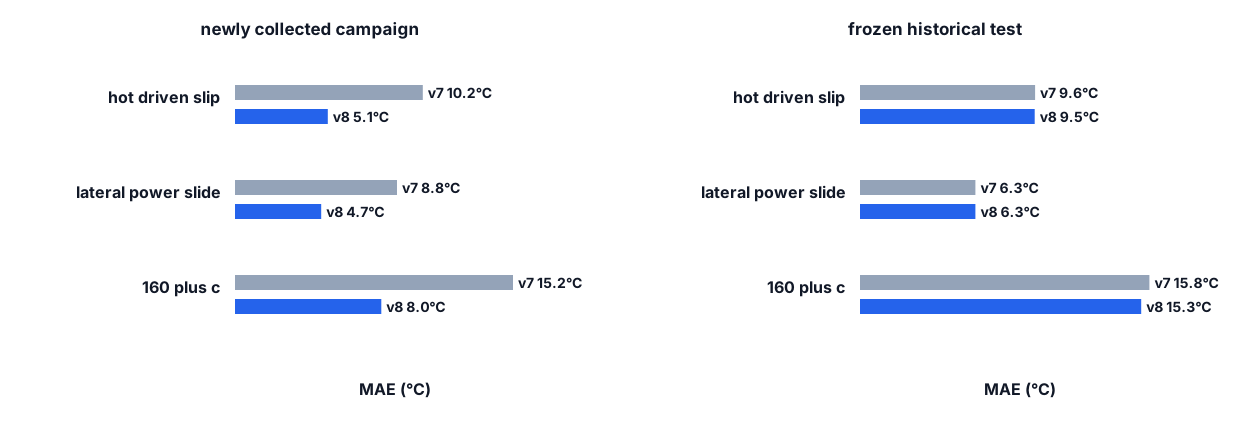
This was probably the most satisfying result of the project. The improvement wasn’t coming from another architecture or a clever loss function. It came from understanding where the model failed, deliberately creating more examples of those situations, and seeing the errors move in response.

It also confirmed the slightly annoying implication: getting substantially better probably meant doing more of exactly that.

What didn’t fix it

I tried a bunch of other ideas at the training level, but none of them really changed the picture. Some helped around the edges, but the fundamental problem remained: there still weren’t enough examples of the difficult regimes for the model to learn them reliably.

The useful results, in short (MAE figures are approximate; only compare models evaluated on the same frozen split):

• Sampling: 10 Hz aggregate matched or beat 30 Hz in the screening runs (roughly 3.9°C validation MAE) with sequences one third as long. A 5-second window stride beat 15 seconds by 0.36–0.48°C.
• Training windows: 35% event-centred oversampling and left/right mirroring each reduced validation MAE from 3.45°C to about 3.40°C. Combined with random window starts they reached 3.25°C; random starts alone reached 3.63°C.
• Loss: Smooth L1 without hot-event oversampling produced the best overall result in that sweep at 3.22°C test MAE. MSE with 35% hot windows was slightly worse overall at 3.27°C, but reduced the 100–120°C and 120–160°C bands to 10.83°C and 13.94°C respectively. Increasing oversampling further was not consistently useful.
• Architecture: On the frozen v8 split, GRU, LSTM and TCN reached 2.95°C, 3.03°C and 2.95°C. The TCN reduced RMSE from 5.62°C to 5.01°C, but not MAE. On the later v12 split, a similarly sized Transformer reached 6.53°C against 2.78°C for the GRU.
• Extra inputs: Tyre-service distance, track surface, location plus altitude, and winsorised normalisation all finished between 2.84°C and 2.98°C on v12, behind the 2.78°C baseline.
• Optimisation and delay: Learning-rate schedules, weight decay and seeds moved the result by roughly 0.1–0.2°C without a stable winner. Giving the model 0.5 seconds of future telemetry changed MAE from 3.034°C to 3.028°C, which was not enough to justify stale inference.

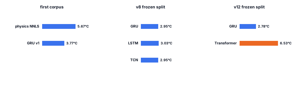
There is always another knob to turn on a neural network. More capacity. Different losses. Longer context. More aggressive weighting of difficult samples. Different feature representations.

Some of those can absolutely matter, and I’m sure the current model is not globally optimal. But once several substantially different training approaches keep struggling with the same small set of behaviours, continuing to tweak the optimizer starts to feel like avoiding the more obvious explanation.

The model cannot learn examples it has never really seen.

And even when it has seen a regime three or four times, that’s not necessarily enough for it to understand the general rule rather than memorize the particular circumstances of those events.

At that point, the best next step was simply to stop forcing the dataset and let new regimes accumulate naturally as I raced.

That is also much closer to the final distribution I actually care about. Instead of spending evenings inventing increasingly bizarre ways of overheating tyres, I can keep recording normal racing sessions and gradually collect the mistakes, unusual setups, tracks and situations that happen naturally.

The model can then improve alongside the dataset rather than turning data generation into a second job.

Where it stands

Final GRU checkpoint: 2.785°C MAE · 5.040°C RMSE · 8.380°C P95 absolute error

The interesting result for me isn’t really that a GRU can predict a temperature curve. Given enough data, that part is not particularly surprising.

What I found much more interesting was how quickly the project stopped being about choosing a model.

The initial physics baseline established that the signal was there. The GRU showed that much richer temporal behaviour could be learned from the live telemetry. And then the remaining failures increasingly mapped back to which parts of the driving distribution I had actually managed to collect.

That is perhaps the useful general lesson from the exercise: sometimes the difficult part of an ML problem is not making the model more sophisticated, but figuring out what information will actually exist at inference time and making sure your dataset contains enough examples of the situations where the model most needs to work.

For now, my AI Bono will have to keep learning as I do.

Future work

There are still a few parts of the problem I haven’t explored properly. The biggest one is how precisely iRacing models interactions with different surfaces — asphalt, kerbs, grass and gravel — and whether thermal behaviour meaningfully varies between tracks or even between differently surfaced sections of the same track. In real motorsport those differences matter; whether they’re represented strongly enough in iRacing to matter to the estimator is something I’ll leave for future analysis.

A straightforward first experiment would be to compare otherwise similar thermal events across tracks and surface types, while controlling as much as possible for speed, load and driving inputs. If a meaningful residual remains consistently associated with the track or surface, then that probably deserves to become an explicit part of the model.

Another question is generalization between cars. Different tyre constructions, vehicle masses, aero loads and suspension geometries should produce substantially different thermal behaviour. Whether one model can learn enough shared structure to transfer between cars, or whether the practical solution is simply a model per car, is something I haven’t investigated yet.

Appendix: Session boundaries and resets

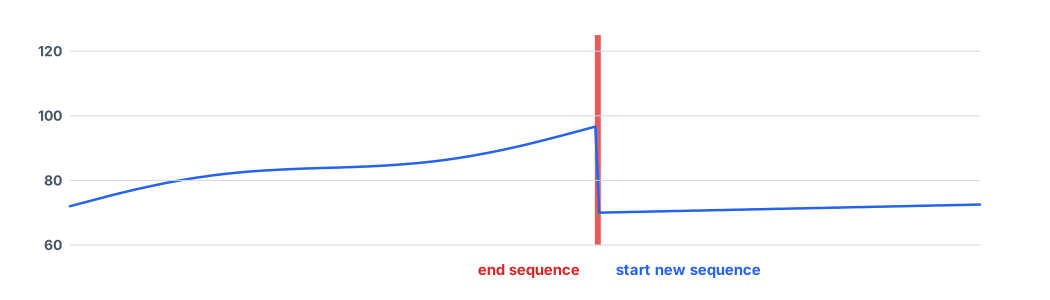
Session boundaries and tyre resets. Defining training sessions/chunks has one annoying iRacing-specific wrinkle. In practice sessions I sometimes disable damage to avoid repeatedly restarting from the garage after a crash, but certain resets also reset tyre temperatures. That’s obviously not thermal behaviour we want the model to learn, so these discontinuities have to be detected and handled outside the model.

For a recurrent model this matters even more than it would for ordinary tabular training data. If a sequence contains 110°C immediately followed by an artificial reset to 60°C, the network has no way to know that iRacing teleported the car back to the pits unless I explicitly provide that information. From its perspective, this is just another thermal transition it is expected to reproduce.

The clean solution is therefore to treat these events as hard sequence boundaries. The recurrent state should be reset, and samples on opposite sides of the event should never be presented as one continuous physical trajectory.